Introduction
Excessive frost heave or settlements are major design and operational issues for hydrocarbon pipelines in permafrost regions. A chilled gas pipeline may lead to frost heave, while a warm oil pipeline may cause degradation of the permafrost resulting in excessive settlement. This example illustrates how TEMP/W can be used to model the changing thermal regime from a pipeline. The TEMP/W results are benchmarked against results published by Coutts and Konrad (1994).
Background
Coutts and Konrad (1994) studied the extent of freezing around a pipe using what is called a “Node State” Finite Element Method. They presented the result shown in Figure 1 and computed that after two years the freezing front would be about 0.6 m and 0.23 m below and beside the pipe invert, respectively.
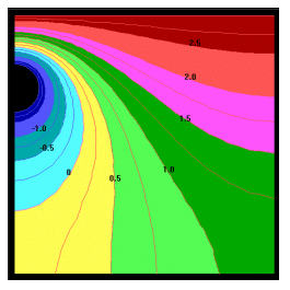
Figure 1. Temperature contours published by Coutts and Konrad (1994).
Numerical Simulation
The model domain for this example is shown in Figure 2. Even though the solution is symmetrical about the central axis, both sides of the symmetry are included in the domain. The main reason for this is that the finite element meshing algorithm gives a nicer concentric mesh around a circular opening representing the pipe. A uniform concentric mesh promotes convergence as the freezing front propagates outward from the circular opening.
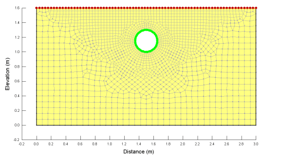
Figure 2. Problem configuration.
Only one transient analysis was used in this example. The centre of the pipe is located at a distance of 1.5m and height of 1.15m, with a radius of 0.15m. The initial temperature of the domain was activated at 3°C such that a steady-state Parent analysis was not required.
The Full Thermal model was used, requiring thermal conductivity and unfrozen volumetric water content (UVWC) functions (Figure 3). The unfrozen and frozen volumetric heat capacities are defined as 1950 kJ/m3 /°C. The in situ volumetric water content was set to 0.3772.
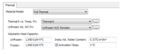
Figure 3. Full Thermal material model dialog box.
The thermal conductivity function was estimated using the Silty Clay sample material with frozen and unfrozen conductivities of 1.8 and 1.5 J/sec/m/°C, respectively (Figure 4). The unfrozen water content function was estimated using the Silty Clay sample material (Figure 5). This curve depicts the portion of the water that freezes as the temperature drops below zero. Most of the water freezes between 0°C and -0.2°C, but a small amount remains unfrozen at temperatures less than -0.2°C.
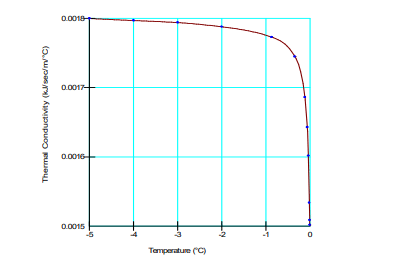
Figure 4. Thermal conductivity function for the Silty Clay material.
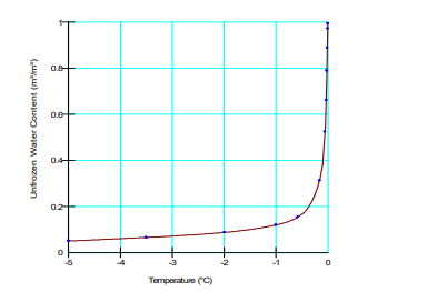
Figure 5. Unfrozen water content function for the Silty Clay material.
The surface of the domain is defined using a constant temperature boundary condition of 3°C. A second constant temperature boundary condition was used to define the temperature of the pipeline and is set to a constant -2°C.
The global element size was set to 0.4 m in the Draw Mesh Properties window (Figure 6). The left, right and bottom boundaries were set to a ratio of 2 of this default size, resulting in an approximate element size of 0.08 m. The circular line representing the pipeline was set to half of the global element size, resulting in an approximate element size of 0.02 m.
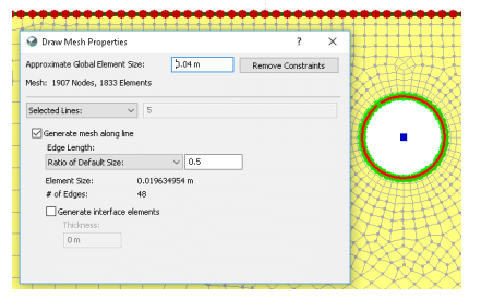
Figure 6. Mesh element size and refinement properties for the line representing the pipeline.
The analysis has 20 time steps for a total duration of 730 days. The time steps increase exponentially with an initial increment size of 1 day. To decrease file size, only every second time step is saved to the file.
Results and Discussion
The resulting thermal conditions after a simulation time of 2 years are shown in Figure 8. The form and shape of the contours are similar to those published by Coutts and Konrad (1994). The TEMP/W solution gives the depth of the freezing front below the pipe invert at 0.65 m, which is similar to the 0.60 m estimate given by Coutts and Konrad (1994). The freezing front width simulated in TEMP/W is the same as Coutts and Konrad (1994), with approximately 0.23 m spread to the right of the pipe invert.
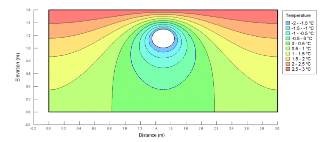
Figure 8. Resulting temperature contours after a simulation time of 2 years.
Any noticeable differences are the result of the meshing and mesh refinement. Figure 9 shows the changing position of the freezing front with time. This diagram can be created with the Draw Isoline command.
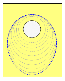
Figure 9. Isolines showing the changing freezing front with time.
Summary and Conclusions
The objective of this example was to illustrate how TEMP/W can be used to simulate the freezing front propagation around a pipeline. The example demonstrates the use of circular regions and the application of the appropriate boundary conditions and material properties.
Reference
Coutts, R.J. and Konrad, J.M. (1994). Finite Element Modeling of Transient Non-Linear Heat Flow Using the Node State Method, International Ground Freezing Conference, France